Differentiable Physical Modeling for Parameter Estimation

Jin Woo Lee

Objectives

• Categorize existing approaches for parameter estimation in physical modeling
• Interpret the role of differentiable simulation and neural networks
• Estimate control parameters by implementing the differentiable plucked string simulation

Parameter Estimation in Physical Modeling

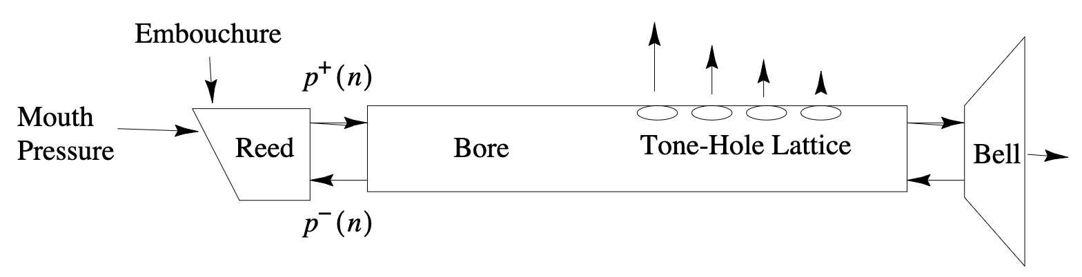
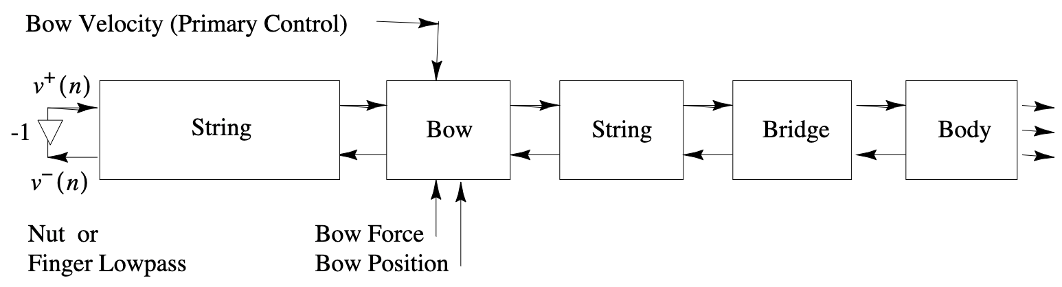
Physical Modeling Sound Synthesis

• Synthesized samples (Smith 1992)
  

Sound examples from https://ccrma.stanford.edu/
    ~jos/waveguide/Sound_Examples.html

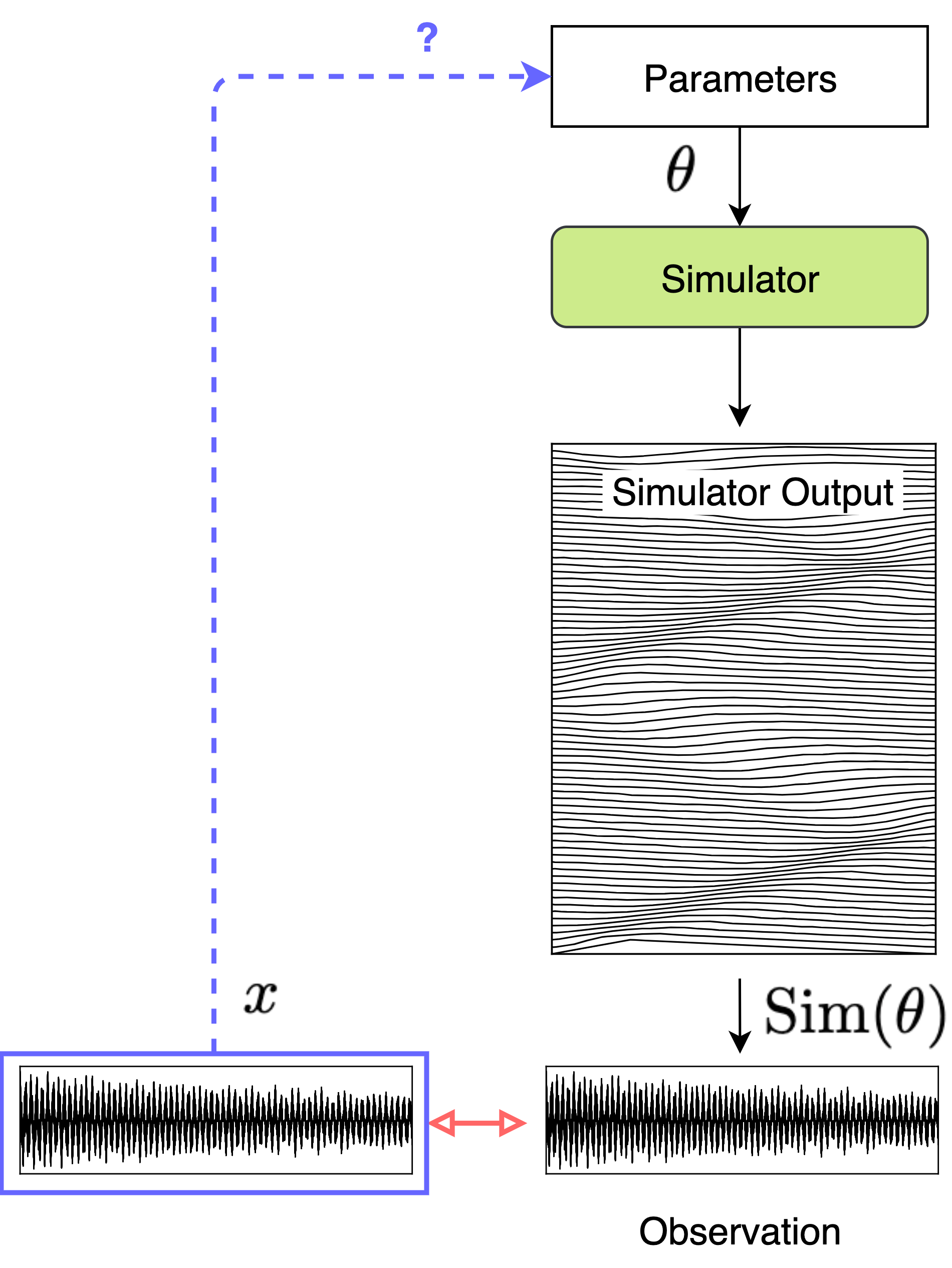
The inverse problem

• Objective:
  • given a known observation (target sound)
  • find the simulator’s input parameters
  • that can closely resemble the target sound.

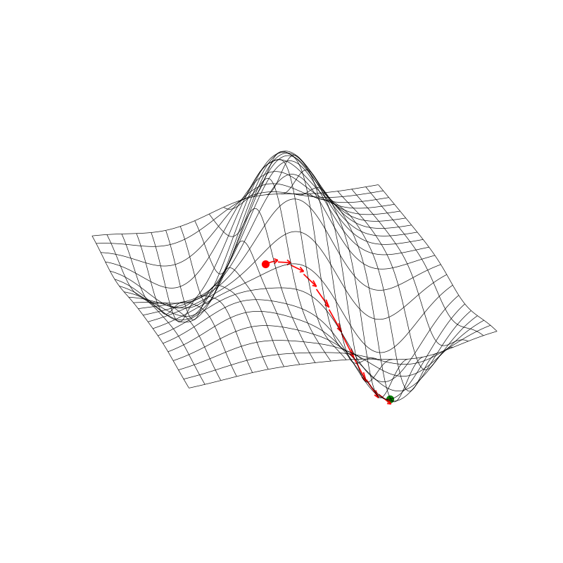
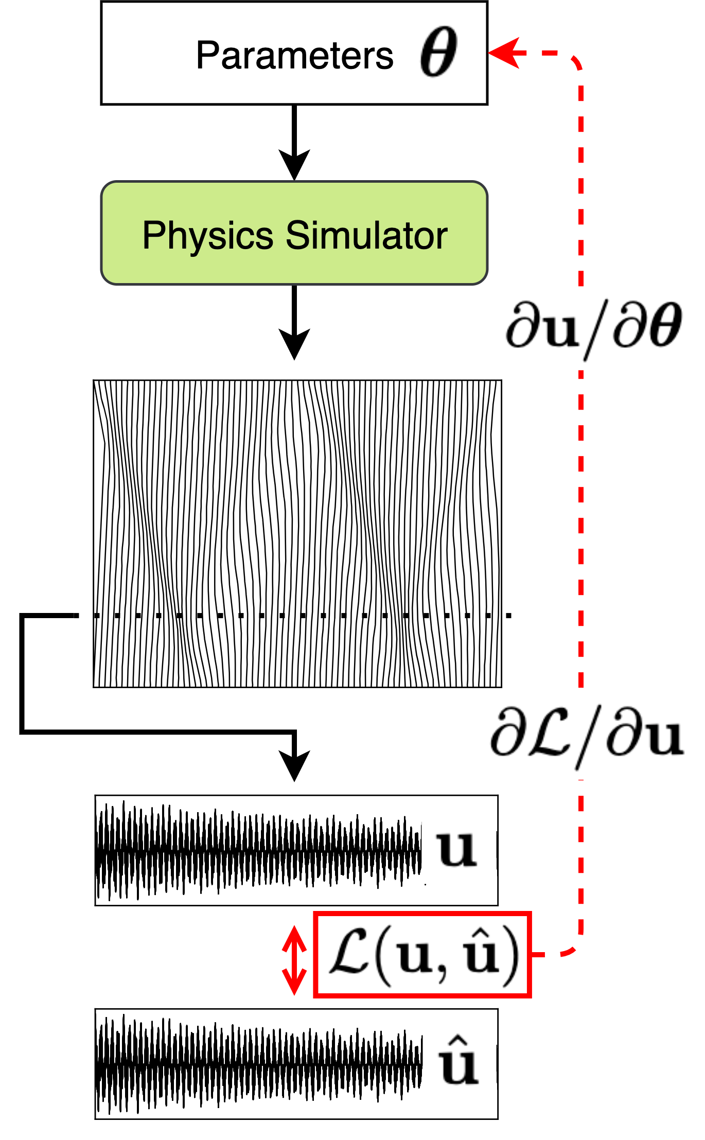
The parameter estimation

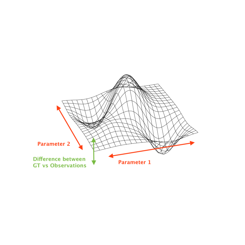
• Point estimation
  • To find the exact parameter “data point”
  • cf. frequentist interpretation

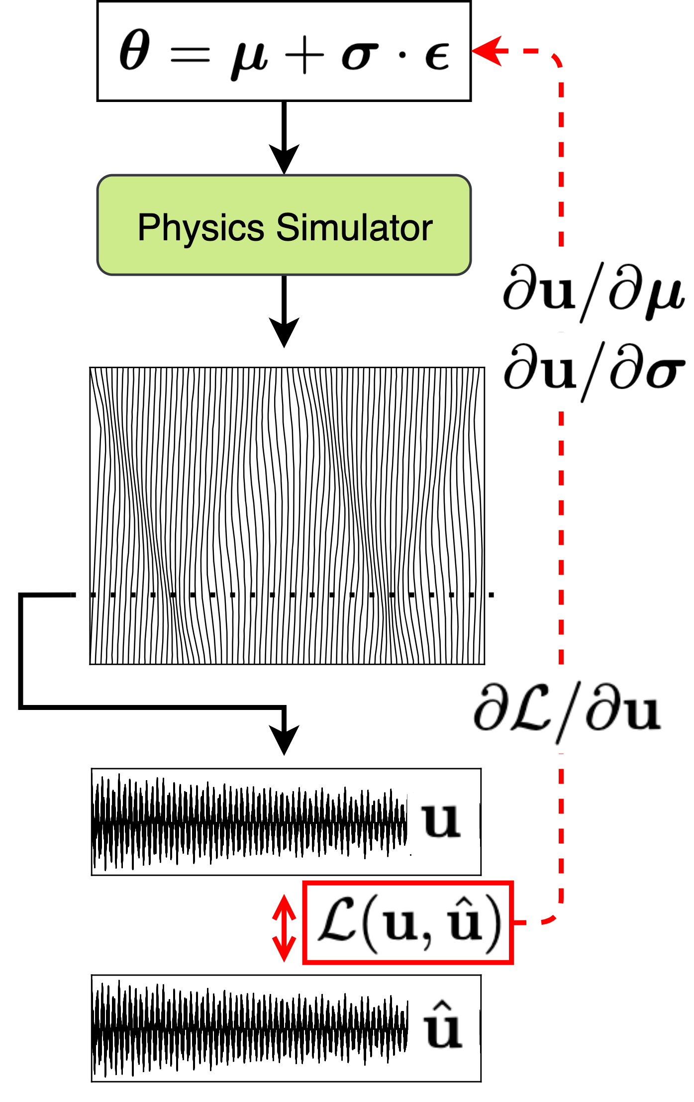
• Distribution estimation
  • To find a generator that can draw parameter “set”
  • cf. Bayesian interpretation

Differentiable Simulation for Parameter Estimation

FDTD Example (1D Wave Equation)

The 1D wave equation with a point source excitation \[ \frac{\partial^2 u}{\partial t^2} = \gamma^2 \frac{\partial^2 u}{\partial x^2} + \delta(x - x_F)\cdot f_\tau(t - t_F) \]

• \(x_F=\) excitation location, \(f_\tau(t - t_F)=\) excitation signal

\[ \mathbf{U}[t_{+\Delta t}] = \left(2\mathbf{I} + \lambda^2\mathbf{D}_{xx} \right) \mathbf{U}[t] - \mathbf{U}[t_{-\Delta t}] + (\Delta t)^2 \mathbf{E}_{ii}\mathbf{f}[t] \]

• Grid points: \(N_x,N_t\)
• \(\mathbf{E}_{ii} = \mathbf{e}_i\mathbf{e}_i^\top \in \mathbb{R}^{N_x \times N_x}\)
• \(\mathbf{I} \in \mathbb{R}^{N_x \times N_x}\)
• \(\mathbf{D}_{xx} \in \mathbb{R}^{N_x \times N_x}\): 2nd order difference
• \(\mathbf{U}[t] := [\mathbf{u}[t, x_1], \mathbf{u}[t, x_2], \ldots, \mathbf{u}[t, x_{N_x}]]^\top \in \mathbb{R}^{N_x}\)

FDTD Example (1D Wave Equation) \(x_F\)

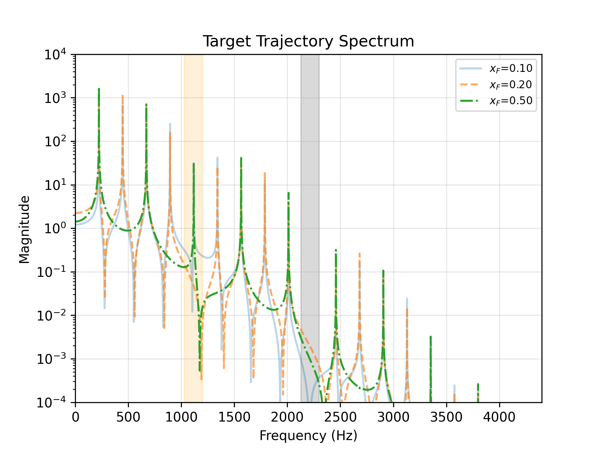
Spectrum of the string with \(F_0=220\) Hz, output picked up at \(x=0.5\)

Forcing location \(x_F\)

• \(x_F=0.1\)
  Missing \(10 n\times F_0\)
• \(x_F=0.2\)
  Missing \(5 n\times F_0\)
• \(x_F=0.5\)
  Missing \(2 n\times F_0\)

FDTD Example (1D Wave Equation) \(t_F\)

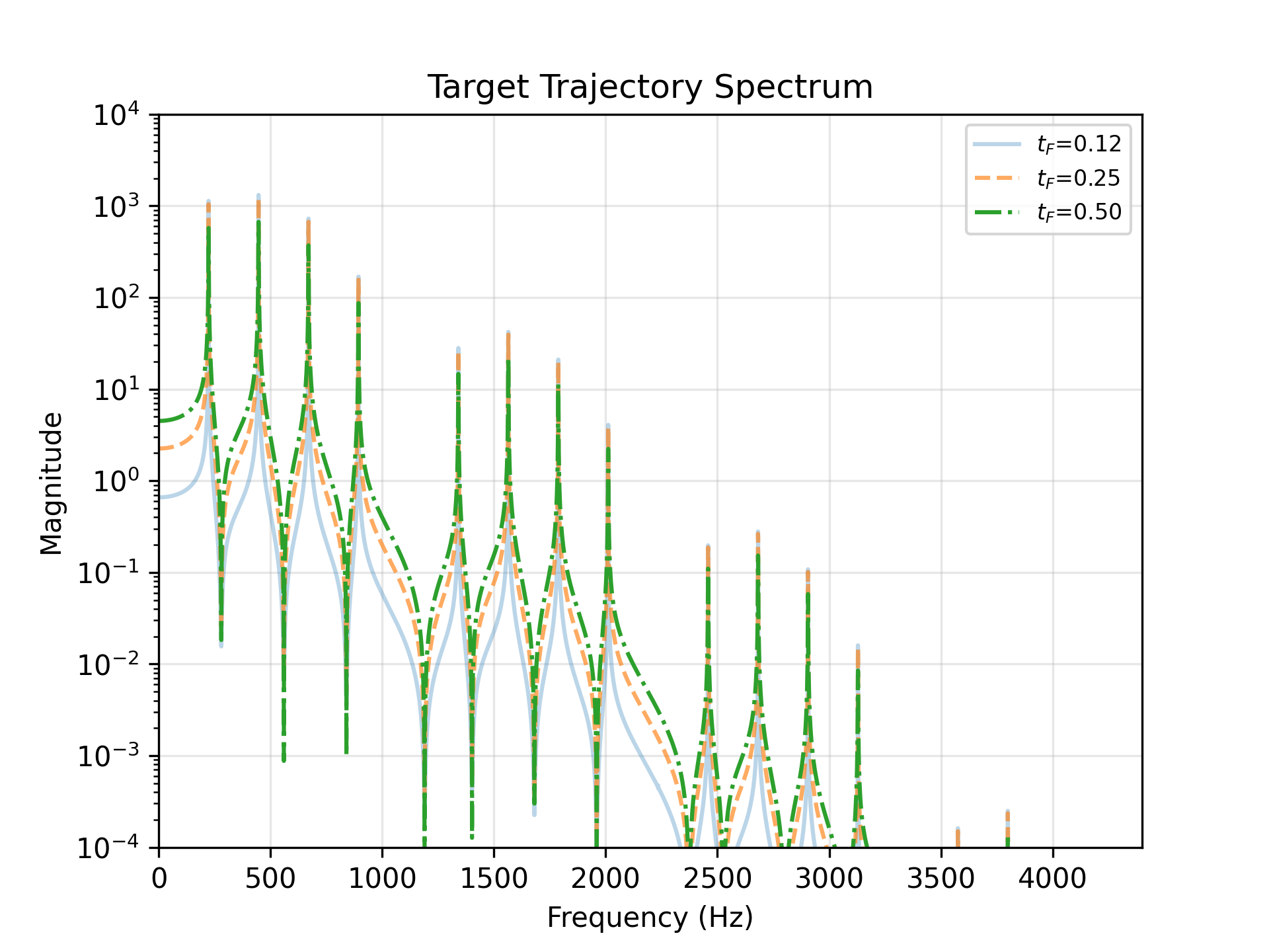
Forcing onset time \(t_F\)

• \(t_F=0.12\)
• \(t_F=0.25\)
• \(t_F=0.50\)

FDTD Example (1D Wave Equation) \(\tau\)

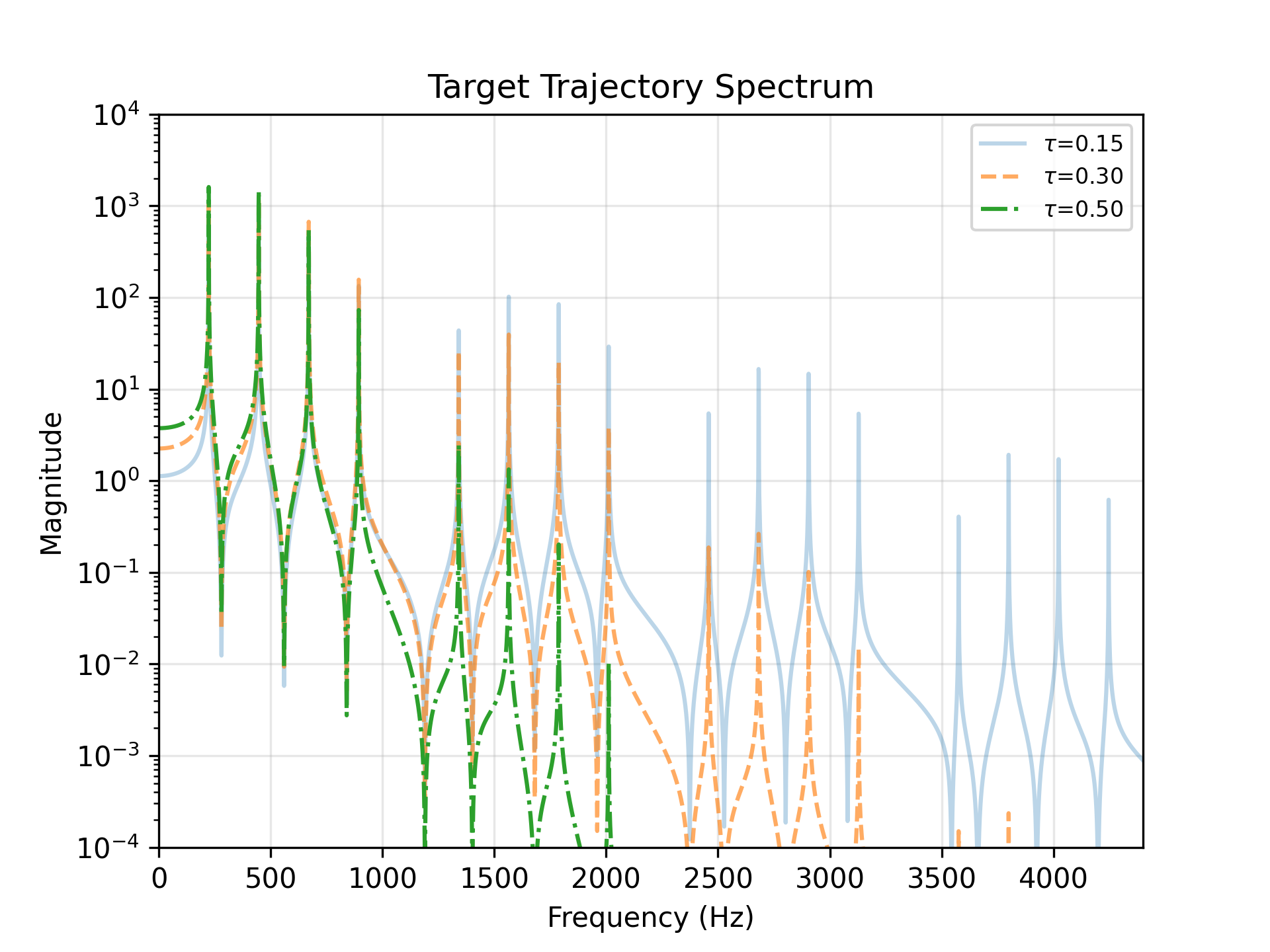
Forcing duration \(\tau\)

• \(\tau=0.15\)
• \(\tau=0.30\)
• \(\tau=0.50\)

Point Estimation using Diff. FDTD

• Given:
  • Target observation \(\mathbf{\hat{u}} \in \mathbb{R}^{N_t}\)
  • Differentiable simulator (e.g., FDTD simulation)
    • excitation parameterized by \(\boldsymbol{\theta} = [x_F, t_F, \tau]\) where \(f_\tau(t - t_F) = \exp\!\left( - \frac{(t - t_F)^2}{2\tau^2} \right)\)
    • \(\boldsymbol{\theta}\) randomly initialized in a reasonable range
• Objective:

  • Find the optimal parameter \(\boldsymbol{\theta}^*\)

    \[ \boldsymbol{\theta}^* = \arg\min_{\boldsymbol{\theta}} \left\|\mathbf{u}(\boldsymbol{\theta}) - \mathbf{\hat{u}}\right\| \]

    that can reproduce the target observation.

Point Estimation: Result 1

Two observation positions

• Estimated
  • (left): \(x_F\) position
  • (right): entire time-space trajectory
    
    
    
• at observation 1
  • (left): gt vs est
  • (right): time-error
    
    
    
    
• at observation 2
  • (left): gt vs est
  • (right): time-error

Point Estimation: Result 2

Different initializations on the parameters, subject to a single observation

• The optimization can lead to different solutions

Distribution Estimation using Diff. FDTD

• Given:
  • Target observation \(\mathbf{\hat{u}} \in \mathbb{R}^{N_t}\)
  • Differentiable simulator (e.g., FDTD simulation)
    • Same excitation parametes \(\boldsymbol{\theta} = [x_F, t_F, \tau]\)
    • But sampled from a certain distribution
• Objective:

  • Find the optimal \(\phi^*\) that \(\boldsymbol{\theta}\sim\boldsymbol{q}_{\phi^*}\)

    \[ \phi^* = \arg\min_{\boldsymbol{\phi}} \mathbb{E}_{\theta\sim\boldsymbol{q}_{\phi}}\left\|\mathbf{u}(\boldsymbol{\theta}) - \mathbf{\hat{u}}\right\| \]

  • \(q_\phi\): parameter sampler (distribution generator)

  • Reparameterize \(\boldsymbol\theta=\boldsymbol\mu + \boldsymbol\sigma\cdot\boldsymbol\epsilon\) where \(\boldsymbol\epsilon\sim N(\mathbf{0}, \mathbf{I})\)

Distribution Estimation: Result 1

Two observation positions, sample eight \(\theta\)-s every iteration

Distribution Estimation: Result 2

One observation position, optimize two distribution modes

Distribution Estimation: Moving forward

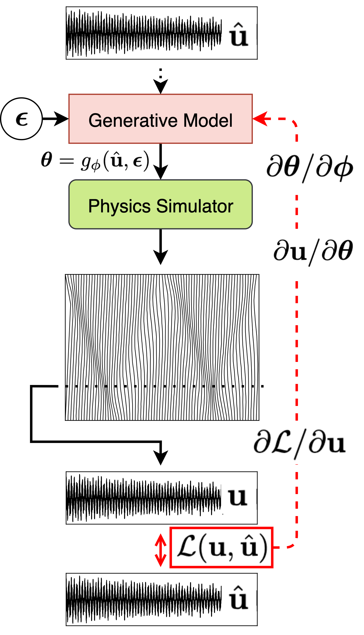
• Being able to compute \(\nabla_\theta \log p(u|\theta)\) can imply many
  applicability in Bayesian methods
  • Markov Chain Monte Carlo (MCMC)
  • Hamiltonian Monte Carlo (HMC)
  • Sequential Monte Carlo (SMC)
• Utilizing real-measured \(\theta\)
  • Securing a good initialization (critical!)

Programming Excercises

Link to the Codes

• Scan the QR code
• Or, access the same link by typing:
  https://bit.ly/ismir-pm-pt4-notebook

• You can also find the same link by doing:
  • type https://ismir-physical-modeling.github.io/ in your browser,
  • scroll down to Schedule,
  • locate to current section (Differentiable … Parameter Estimation),
  • click </> Notebook.

Remarks and Perspectives

Key Takeaways

• There can be multiple possible solutions for an inverse problem with given (partial) observations. (Kac 1966)
• Can use GD to backpropagate through the physical model to update the input parameters.
  • Could be point estimation or distribution estimation.
  • There can be many other approaches other than GD.
• Impelmentation choices: PyTorch, JAX, DiffTaichi (Hu et al. 2020)
• By design, the outputs of all possible solutions are physically plausible.

Perspectives

• Can be challenging to backpropagate through complicated models, possibly due to:
  • Sub-iterations for nonlinear models (Lee et al. 2024)
    • Implicit FDTD schemes, nonlinear scattering junctions
  • Audio sample-rate recursions
    • Gradient vanishing (Zheleznov et al. 2025)
  • Operations that yields harsh non-smoothness (discontinuous derivatives)
    • Friction, collisions, etc.
• Can be extended to improved models with a diverse optimization criteria (Diaz and Sandler 2025)

References

Diaz, Rodrigo, and Mark Sandler. 2025. “Fast Differentiable Modal Simulation of Non-Linear Strings, Membranes, and Plates.” In 28th International Conference on Digital Audio Effects.

Hu, Yuanming, Luke Anderson, Tzu Mao Li, Qi Sun, Nathan Carr, Jonathan Ragan-Kelley, and Frédo Durand. 2020. “DiffTaichi: Differentiable Programming for Physical Simulation.” In 8th International Conference on Learning Representations, ICLR 2020.

Kac, Mark. 1966. “Can One Hear the Shape of a Drum?” The American Mathematical Monthly 73 (4P2): 1–23.

Lee, Jin Woo, Jaehyun Park, Min Jun Choi, and Kyogu Lee. 2024. “Differentiable Modal Synthesis for Physical Modeling of Planar String Sound and Motion Simulation.” Advances in Neural Information Processing Systems 37: 1058–81.

Smith, Julius O. 1992. “Physical Modeling Using Digital Waveguides.” Computer Music Journal 16 (4): 74–91.

Zheleznov, Victor, Stefan Bilbao, Alec Wright, and Simon King. 2025. “Learning Nonlinear Dynamics in Physical Modelling Synthesis Using Neural Ordinary Differential Equations.” In 28th International Conference on Digital Audio Effects, 1–8.